Previously we have written the parametric line equation (where $A$ and $B$ represent points) as $L(t)=A+t(B-A)$. However, we could easily factor it differently. $$L(t)=(1-t)A+tB \tag{1} \label{1}$$

Because points $A$ and $B$ have two components each in $\mathbb{R}^{2}$, $(A_{x},A_{y})$ and $(B_{x}$, $B_{y})$ the equation is parametric. $$L(t)=\left(\begin{array}{c} x\\ y \end{array}\right)=\left(\begin{array}{c} (1-t)A_{x}+tB_{x}\\ (1-t)A_{y}+tB_{y} \end{array}\right) \tag{2} \label{2}$$ We draw a line, $L(t)$, from point $A$ to $B$. Now let's change the variable names and set up a new situation. Start with points $P_{0}$ and $P_{2}$. We can write a line segment equation that connects the two points. Remember, it is a segment because $0 \le t \le 1$ $$L(t)=\left(\begin{array}{c} x\\ y \end{array}\right)=(1-t)P_{0}+tP_{2}\qquad0\le t\le1. \tag{3} \label{3}$$ Now let's create another point, $P_{1}$ and put it anywhere except on the line between $P_{0}$ and $P_{2}$. Next we will write two line equations serially, one from $P_{0}$ to $P_{1}$ and the other from $P_{1}$ to $P_{2}$. See figure 1. $$\begin{array}{c} \left(\begin{array}{c} x_{0}\\ y_{0} \end{array}\right)=(1-t)P_{0}+tP_{1}\\ \\ \left(\begin{array}{c} x_{1}\\ y_{1} \end{array}\right)=(1-t)P_{1}+tP_{2} \end{array} \tag{4} \label{4}$$

Now suppose that we wanted to take the two new points, $(x_{0},y_{0})$ and $(x_{1},y_{y})$ and connect them too with a linear interpolation equation. That equation would be $$\left(\begin{array}{c} x_{2}\\ y_{2} \end{array}\right)=(1-t)\left(\begin{array}{c} x_{0}\\ y_{0} \end{array}\right)+t\left(\begin{array}{c} x_{1}\\ y_{1} \end{array}\right). \tag{5} \label{5}$$ If we did that at $t=0,.1,.2,.3\ldots,1$ we would get string art.

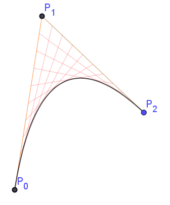
What we will do next is to re-write equation $\bbox[darkblue]{\eqref{3}}$ and substitute for $P_{0}$ and $P_{2}$ the two equations of $\bbox[darkblue]{\eqref{4}}$. Essentially, we will be doing a linear interpolation between a linear interpolation. $$L(t)=\left(\begin{array}{c} x\\ y \end{array}\right)=(1-t){\color{green}\left[(1-t)P_{0}+tP_{1}\right]}+t{\color{blue}\left[(1-t)P_{1}+tP_{2}\right]}\qquad 0\le t\le1\tag{6} \label{6}$$ Equation $\bbox[darkblue]{\eqref{6}}$ now graphs as the black curve in figure 3. Although only marginally better, the equation simplifies to $$L(t)=\left(\begin{array}{c} x\\ y \end{array}\right)=(1-t)^{2}P_{0}+2(1-t)\cdot t\cdot P_{1}+t^{2}P_{2} \tag{7} \label{7}$$

Following the form of equation $\bbox[darkblue]{\eqref{7}}$ we can extend the number of interim points indefinitely. The next one is called a cubic Bèzier and is written as $$(1-t)^{3}P_{0}+3(1-t)^{2}tP_{1}+3(1-t)t^{2}P_{2}+t^{3}P_{3}. \tag{8} \label{8}$$ When $t$ is zero, the curve will be at $P_0$ and when $t=1$ the curve will be at $P_3$. Any other values of $t$ between $0$ and $1$ will cause the curve to be influenced by $P_1$ and $P_2$.